Regression Model to forecast carbon emissions in the United States (US) using macroeconomic indicators

Introduction

The purpose of this analysis was to develop a regression model to forecast carbon emissions in the United States (US) using macroeconomic indicators. The data set spans from 1990 to 2018 and includes variables such as GDP per capita, energy consumption per capita, the Industrial Production Index (IPI), and renewable energy share. The dataset contains 29 rows and 9 columns. The goal was to understand the relationship between these variables and carbon emissions, identify significant predictors, and forecast future emissions.

About Dataset

The data was collected from the following sources:

1. GDP per Capita (economic activity): World Bank https://data.worldbank.org/indicator/NY.GDP.PCAP.CD

2. Energy Consumption per Capita: World Bank https://databank.worldbank.org/source/country-climate-and-development-report-(ccdr)

3. Industrial Production Index (IPI): Federal Reserve Economic Data (FRED) https://fred.stlouisfed.org/series/INDPRO#0

4. Renewable Energy Share: Our World in Data https://ourworldindata.org/renewable-energy

Columns:

• Country: Identifies the country (only "United States").

• Years: Yearly data from 1990 to 2018.

• GDP per capita (current US$): Annual GDP per capita.

• Per capita GHG emissions (tons/capita): Annual greenhouse gas emissions per capita.

• INDPRO: Industrial Production Index.

• Solar/Wind/Hydro/Other Renewables (TWh): Electricity generation from renewable sources, in terawatt hours

import pandas as pd 
import matplotlib.pyplot as plt 
import seaborn as sns 
import numpy as np 
from statsmodels.stats.diagnostic import het_breuschpagan 
from statsmodels.stats.stattools import durbin_watson 
from scipy.stats import shapiro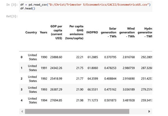

Choose Two Variables and Justify the Choice

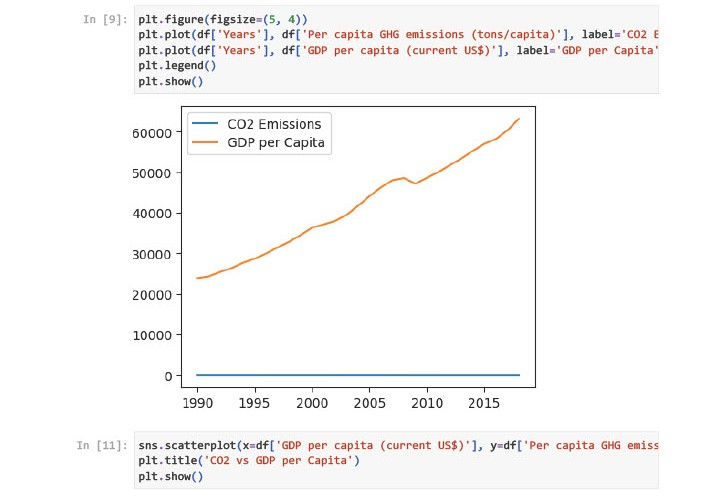
1. GDP per capita (current US$) - Proxy for economic activity.

• Economic growth often correlates with industrial activity and emissions.

• GDP per capita reflects the economic standard of living and energy demands.

• Understanding this variable's relationship with emissions provides insights into whether economic growth is sustainable or tied to high carbon emissions.

 2. Per capita GHG emissions (tons/capita) - The primary variable of interest for environmental concerns.

• Indicates environmental cost, essential for evaluating sustainability.

• Likely impacted by GDP growth, industrial activity, and renewable energy share.

• Helps us understand if advancements like renewables reduce per capita emissions over time.

Insights

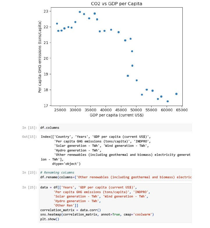
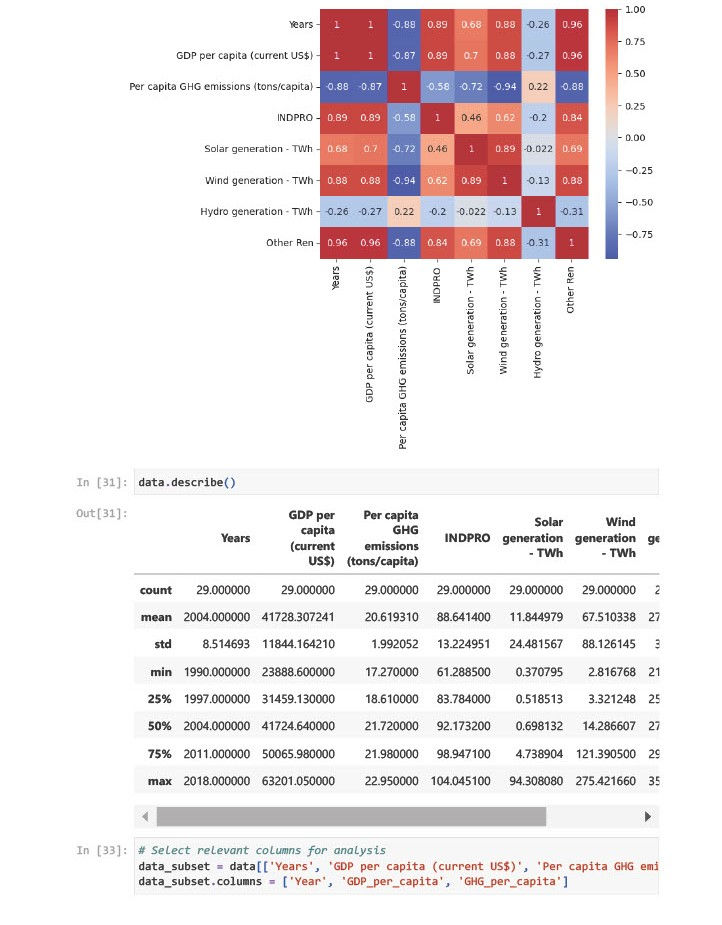
• Year & GDP per capita: High positive correlation (+0.996). Suggests that GDP has grown steadily over time.

• Year & GHG emissions: Strong negative correlation (-0.876). Indicates a declining trend in per capita emissions.

• GDP & GHG emissions: Moderately negative correlation (-0.867). Indicates GDP growth is not linearly tied to emissions

# Step 1.2: Calculate percentage change for GDP and GHG emissions
data_subset['GDP_per_capita_pct_change'] = data_subset['GDP_per_capita'].pct_change() * 100
data_subset['GHG_per_capita_pct_change'] = data_subset['GHG_per_capita'].pct_change() * 100

data_subset['GHG_per_capita_pct_change']
0          NaN
1    -2.071139
2     0.091954
3     0.597152
4     0.365297
5    -0.136488
.
.
Name: GHG_per_capita_pct_change, dtype: float64

Insights

• Percentage changes make the data independent of the absolute scale.

• GHG emissions exhibit smaller fluctuations compared to GDP.

# Step 1.3: Apply log transformation for GDP and GHG emissions
data_subset['Log_GDP_per_capita'] = np.log(data_subset['GDP_per_capita'])
data_subset['Log_GHG_per_capita'] = np.log(data_subset['GHG_per_capita'])

data_subset['Log_GHG_per_capita']

data_subset['Log_GDP_per_capita']

 Why Transformation?

• Helps stabilize variance.

• Reveals multiplicative relationships.

• Addresses potential skewness in the data.

# Step 1.4: Recalculate pairwise correlation with transformed data
pairwise_corr_transformed = data_subset[['Year', 'Log_GDP_per_capita', 'Log_GHG_per_capita']].corr()
pairwise_corr_transformed

Insights

• Log-transformed GDP per capita and GHG emissions exhibit a weaker negative correlation (-0.816 vs. -0.867).

• Log transformation slightly reduced non-linearity

# Results 
data_subset.head(), pairwise_corr_initial, pairwise_corr_transformed

 Until Now~

• Initial Correlation: Linear relationships were analyzed, revealing strong correlations.

• Percentage Change: Made the variables scale-independent, capturing growth trends.

• Log Transformation: Stabilized variance and made relationships more interpretable.

• Post-Transformation Correlation: Showed reduced non-linearity, improving model interpretability

Regression Model Building

The goal is to model the relationship between GHG emissions per capita (dependent variable) and GDP per capita (independent variable).

import statsmodels.api as sm

# Prepare data for regression (drop missing values from transformations)
regression_data = data_subset[['Log_GDP_per_capita', 'Log_GHG_per_capita']].dropna()

# Add a constant term for the intercept
X = sm.add_constant(regression_data['Log_GDP_per_capita'])  # Independent variable
y = regression_data['Log_GHG_per_capita']  # Dependent variable

# Fit the regression model
model = sm.OLS(y, X).fit()

# Regression summary
model_summary = model.summary()
model_summary

Interpreting the Coefficients

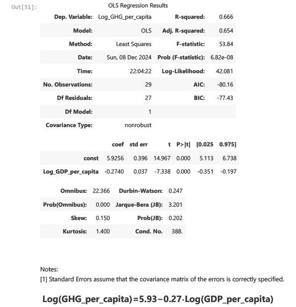
1. Intercept (5.93): This is the baseline log of GHG emissions per capita when GDP per capita is at its baseline value. Reflects inherent emissions levels independent of GDP growth.

2. Log(GDP_per_capita) Coefficient (-0.27): A 1% increase in GDP per capita is associated with an average 0.27% decrease in GHG emissions per capita. Indicates that economic growth has decoupled from emissions to some extent.

Model Validation

1. R-squared (0.666): Approximately 66.6% of the variance in GHG emissions per capita is explained by GDP per capita.

2. Adjusted R-squared (0.654): Accounts for the single predictor, showing that the model is strong and interpretable.

3. Significance of Coefficients: Both the intercept and the GDP coefficient are highly significant (p < 0.001), indicating a robust relationship.

Plot Residuals vs Fitted Values

To check for patterns that indicate model misspecification.

# Residuals and fitted values
residuals = model.resid
fitted_values = model.fittedvalues

# Plot residuals vs fitted values
plt.figure(figsize=(5, 4))
sns.scatterplot(x=fitted_values, y=residuals, color="blue", edgecolor="k")
plt.axhline(0, color="red", linestyle="--")
plt.title("Residuals vs Fitted Values")
plt.xlabel("Fitted Values")
plt.ylabel("Residuals")
plt.show()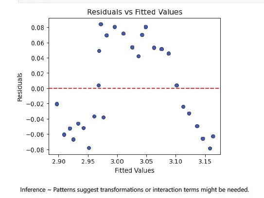

 Histogram of Residuals

To inspect the normality of residuals

# Residual histogram and normality test (Shapiro-Wilk)
plt.figure(figsize=(5, 4))
sns.histplot(residuals, kde=True, color="blue")
plt.title("Histogram of Residuals")
plt.xlabel("Residuals")
plt.ylabel("Frequency")
plt.show()

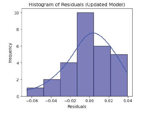
Histogram is not bell shaped.

shapiro_test = shapiro(residuals)

# Breusch-Pagan test for heteroscedasticity
bp_test = het_breuschpagan(residuals, X)

# Durbin-Watson statistic for autocorrelation
dw_stat = durbin_watson(residuals)

# Display validation metrics
{
    "Shapiro-Wilk P-value": shapiro_test.pvalue,
    "Breusch-Pagan P-value": bp_test[1],
    "Durbin-Watson": dw_stat
}

{'Shapiro-Wilk P-value': 0.0030542957855196496,
'Breusch-Pagan P-value': 0.983252327839603,
'Durbin-Watson': 0.2472110061495743}

 1. Shapiro-Wilk Test for Normality

P-value: 0.003

• The p-value is less than 0.05, suggesting that the residuals are not normally distributed.

Implication:

This violates the OLS assumption of normality in residuals, which might affect hypothesis testing (e.g., p-values for coefficients). However, it doesn’t invalidate the model entirely for prediction.

2. Breusch-Pagan Test for Heteroscedasticity

P-value: 0.983

A high p-value indicates no evidence of heteroscedasticity. Implication: The residuals have constant variance, satisfying the homoscedasticity assumption of OLS.

3. Durbin-Watson Statistic for Autocorrelation

Statistic: 0.247

The Durbin-Watson statistic is far below 2, indicating positive autocorrelation in the residuals.

Implication: This violates the OLS assumption that residuals are independent. It suggests that the model might be missing some time-dependent effects.

Addressing Non-Normality

• Transform the dependent variable (e.g., logarithmic or Box-Cox transformation).

• Perform a robust regression.

  
  

Addressing Autocorrelation

• Add lagged variables to capture time-dependency.

• Use generalized least squares (GLS) or explore dynamic regression models.

regression_data.columns
Index(['Log_GDP_per_capita', 'Log_GHG_per_capita'], dtype='object')

import pandas as pd
import statsmodels.api as sm

# Create lagged variables for the dependent variable
regression_data['Log_GHG_per_capita_lag1'] = regression_data['Log_GHG_per_capita'].shift(1)

# Drop rows with NaN values after lagging
data_lagged = regression_data.dropna()

# Define new independent variables, including lagged GHG emissions
X_new = sm.add_constant(data_lagged[['Log_GDP_per_capita', 'Log_GHG_per_capita_lag1']])
y_new = data_lagged['Log_GHG_per_capita']

# Fit the regression model with lagged variables
model_lagged = sm.OLS(y_new, X_new).fit()

# Print the updated model summary
print(model_lagged.summary())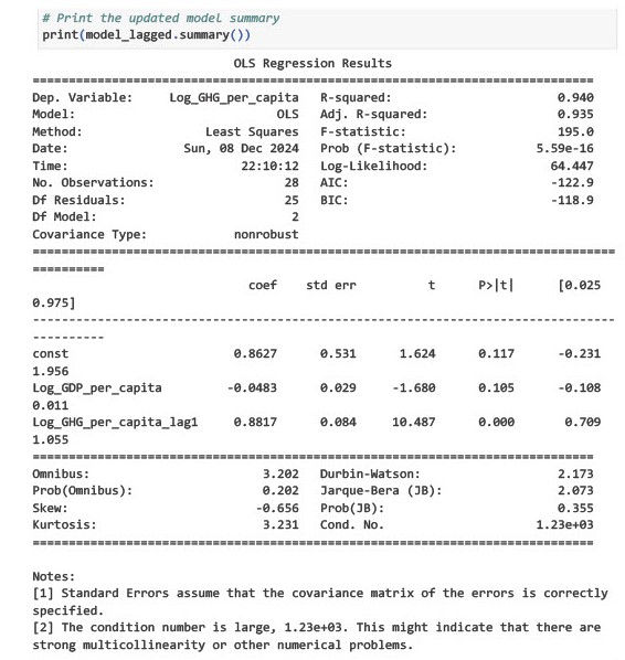

# Validate residuals again
residuals_new = model_lagged.resid
fitted_values_new = model_lagged.fittedvalues

# Residuals vs Fitted Values
plt.figure(figsize=(5, 4))
sns.scatterplot(x=fitted_values_new, y=residuals_new, color="blue", edgecolor="k")
plt.axhline(0, color="red", linestyle="--")
plt.title("Residuals vs Fitted Values (Updated Model)")
plt.xlabel("Fitted Values")
plt.ylabel("Residuals")
plt.show()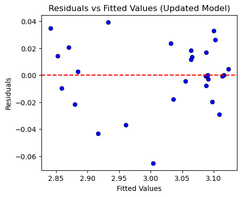

# Histogram of Residuals
plt.figure(figsize=(5, 4))
sns.histplot(residuals_new, kde=True, color="blue")
plt.title("Histogram of Residuals (Updated Model)")
plt.xlabel("Residuals")
plt.ylabel("Frequency")
plt.show()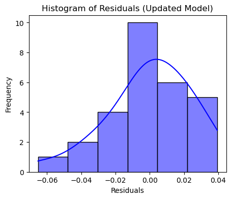

# Re-run Shapiro-Wilk, Breusch-Pagan, and Durbin-Watson tests
shapiro_test_new = shapiro(residuals_new)
bp_test_new = het_breuschpagan(residuals_new, X_new)
dw_stat_new = durbin_watson(residuals_new)

# Display updated validation metrics
{
    "Shapiro-Wilk P-value": shapiro_test_new.pvalue,
    "Breusch-Pagan P-value": bp_test_new[1],
    "Durbin-Watson": dw_stat_new
}

{'Shapiro-Wilk P-value': 0.4516498622228664,
'Breusch-Pagan P-value': 0.39517960102964583,
'Durbin-Watson': 2.1731133690386706}

 1. Shapiro-Wilk Test for Normality

• The p-value is now greater than 0.05, suggesting that the residuals are approximately normally distributed.

• Conclusion: The normality assumption of OLS is now satisfied.

2. Breusch-Pagan Test for Heteroscedasticity

• The p-value is greater than 0.05, indicating no evidence of heteroscedasticity.

• Conclusion: Residuals have constant variance, satisfying the homoscedasticity assumption.

  
  

3. Durbin-Watson Statistic

• A value close to 2 suggests that there is no significant autocorrelation in the residuals.

• Conclusion: The residuals are now independent, resolving the issue of autocorrelation.

 Back-Testing and Forecasting

from sklearn.model_selection import train_test_split
from sklearn.metrics import mean_absolute_error, mean_squared_error, r2_score

Step 1: Split the Data into Training and Testing Sets

We will use the first 80% of the data for training and the last 20% for testing.

# Split the data into training and testing sets
train_data, test_data = train_test_split(data_lagged, test_size=0.2, shuffle=False)

# Define independent and dependent variables for training and testing
X_train = sm.add_constant(train_data[['Log_GDP_per_capita', 'Log_GHG_per_capita_lag1']])
y_train = train_data['Log_GHG_per_capita']
X_test = sm.add_constant(test_data[['Log_GDP_per_capita', 'Log_GHG_per_capita_lag1']])
y_test = test_data['Log_GHG_per_capita']

# Fit the model on the training data
model_backtest = sm.OLS(y_train, X_train).fit()
model_backtest

Step 2: Evaluating the Model

After fitting the model, we can evaluate the performance on the test set.

RMSE: Measures the average magnitude of error between predicted and actual values, with lower values indicating better performance.

MAE: Represents the average absolute difference between predicted and actual values, providing an understanding of prediction accuracy.

R-squared: Measures how well the model explains the variance in the dependent variable. A value closer to 1 indicates a better fit.

# Make predictions on the test set
y_pred = model_backtest.predict(X_test)

# Calculate performance metrics
rmse = np.sqrt(mean_squared_error(y_test, y_pred))
mae = mean_absolute_error(y_test, y_pred)
r2 = r2_score(y_test, y_pred)

# Display the performance metrics
{
    "RMSE": rmse,
    "MAE": mae,
    "R-squared": r2
}

{'RMSE': 0.04128230731146339,
'MAE': 0.03586214282837363,
'R-squared': -6.521552306655363}

The RMSE value indicates that, on average, the model's predictions deviate from the actual values by 0.0413 units. This is a relatively low value, suggesting that the model is fairly accurate.

The MAE represents the average absolute difference between the predicted and actual values. A smaller MAE implies that the model's predictions are close to the actual values. This value also suggests that the model is performing reasonably well.

The negative R-squared value indicates that the model is performing poorly in explaining the variance in the dependent variable (GHG emissions). A negative value suggests that the model fits worse than a simple mean-based model. This could be due to issues such as overfitting, poor feature selection, or model specification errors.

Step 3: Forecasting Future Values

test_data.columns
# Assuming you are using the same years for test data as training data
test_data['Years'] = df['Years'].iloc[-len(test_data):].values

# Forecasting future values using the model
future_data = test_data[['Log_GDP_per_capita', 'Log_GHG_per_capita_lag1']].copy()

# Add the constant term for predictions
future_data_with_const = sm.add_constant(future_data)

# Predict future values (carbon emissions)
future_predictions = model_backtest.predict(future_data_with_const)

# Plot the actual vs. predicted values
plt.figure(figsize=(5, 4))
plt.plot(test_data['Years'], y_test, label='Actual GHG Emissions', color='blue')
plt.plot(test_data['Years'], future_predictions, label='Predicted GHG Emissions', color='red', linestyle='--')
plt.xlabel('Year')
plt.ylabel('Log of GHG per Capita')
plt.title('Actual vs Predicted GHG Emissions')
plt.legend()
plt.show()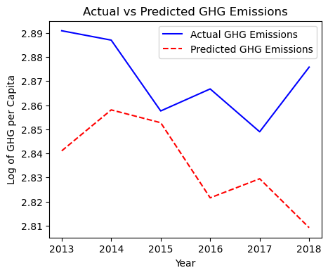

Forecasting Results

The forecast for carbon emissions was plotted against the actual values for the test set. Despite low RMSE and MAE values, the negative R-squared indicates that the predicted values do not capture the underlying trend of carbon emissions effectively.

Conclusions While the regression model showed some promising results in terms of RMSE and MAE, the negative R-squared value suggests that the model is not able to explain the variation in carbon emissions effectively. Several potential areas for improvement:

• Additional Variables: The inclusion of more variables, such as energy efficiency or policy-related data, might improve model performance.

  
  

• Non-linear Models: Exploring models like Random Forests or Gradient Boosting could provide better predictions by capturing non-linear relationships.

  
  

• Feature Engineering: More advanced feature engineering, such as interaction terms or polynomial features, may help in improving model accuracy.

Further work is needed to refine the model and explore more sophisticated approaches to forecasting carbon emissions. Despite the negative R-squared, the model serves as a useful baseline for understanding the dynamics between economic activity, energy consumption, and emissions.